10:00
Week 10 Completed File
Introduction to Basic Modeling

In the second part of the course we will leverage the following resources:
- The Tidy Modeling with R book second portion of the course book
- The Tidy Models website second portion of the course website
Link to other resources
Internal help: posit support
External help: stackoverflow
Additional materials: posit resources
While I use the book as a reference the materials provided to you are custom made and include more activities and resources.
If you understand the materials covered in this document there is no need to refer to other resources.
If you have any troubles with the materials don’t hesitate to contact me or check the above resources.
Class Objectives
Introduce the
tidymodelsframework, highlighting its comprehensive ecosystem designed to streamline the predictive modeling process in R.Establish a foundation of modeling using
tidymodels, emphasizing practical application through the exploration of theamesdataset.
Load packages
This is a critical task:
Every time you open a new R session you will need to load the packages.
Failing to do so will incur in the most common errors among beginners (e.g., ” could not find function ‘x’ ” or “object ‘y’ not found”).
So please always remember to load your packages by running the
libraryfunction for each package you will use in that specific session 🤝
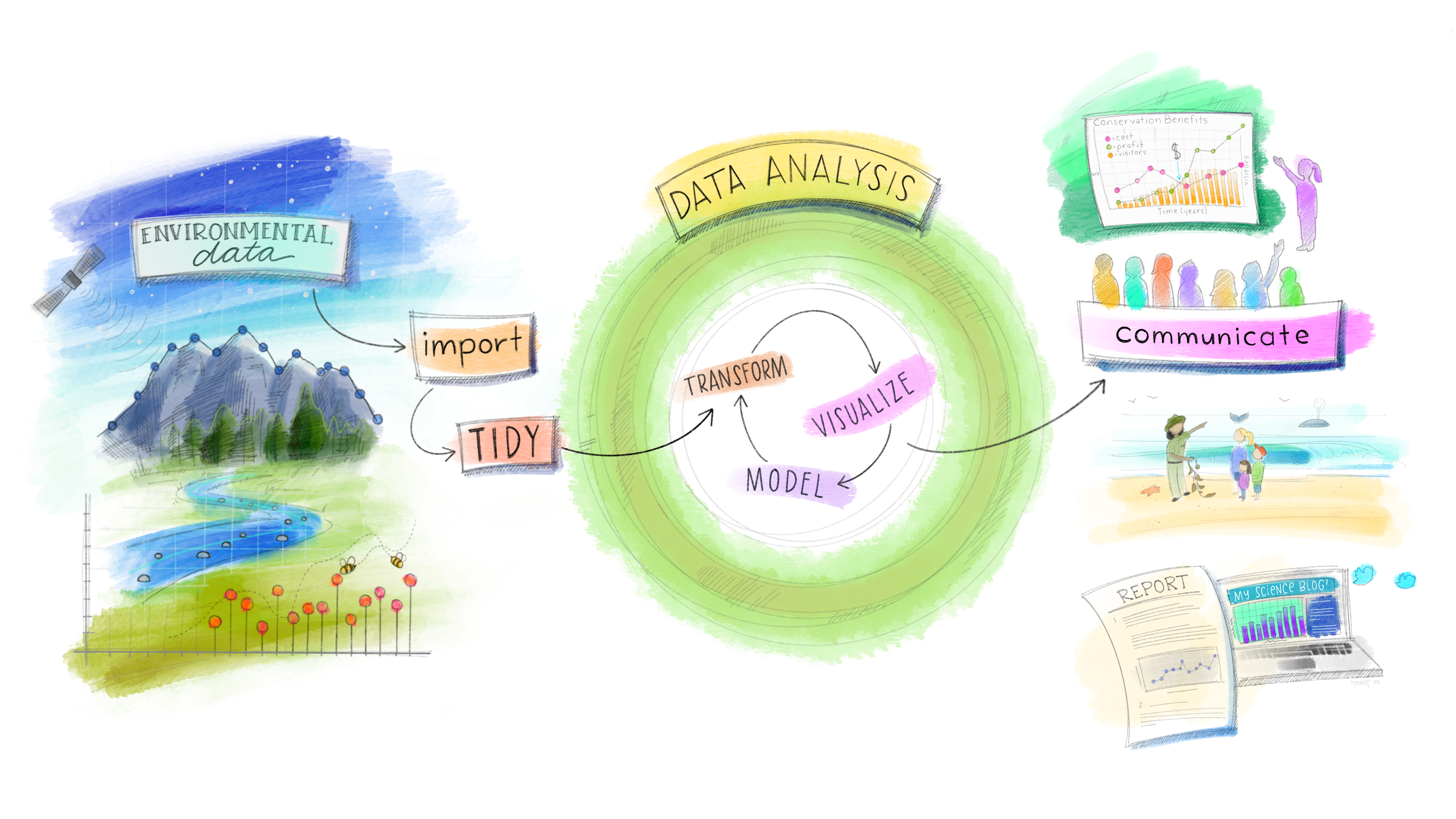
The tidymodels Ecosystem in action
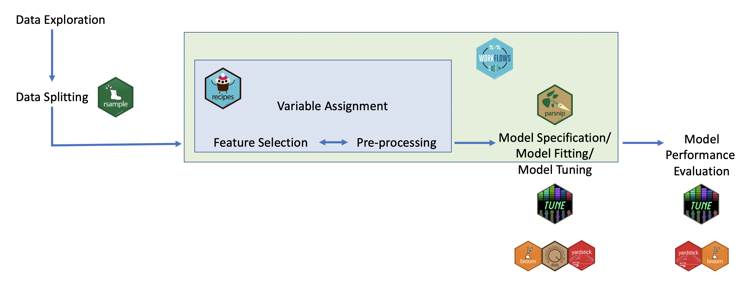
After the theoretical introduction let’s check the tidymodels ecosystem in action, highlighting its components like recipes, parsnip, workflows, etc., and how it integrates with the tidyverse. But first we need to:
Exploring the ames Dataset
The ames housing dataset will be used in this portion of the course. Let’s explore the dataset to understand the variables and the modeling objective (predicting house prices).
Activity 0: Get to know and Explore the ames dataset.
The objective here is to leverage what we learned so far to understand the data. Write all the code you think is needed to complete the task in the chunks below - 10 minutes
Warning
Keep in mind that Sale_Price will be our dependent variable in supervised modeling. Identify possible relevant independent variables by producing charts and descriptive stats. Think also about potential manipulations needed on those variables/creating new variables.
The ames housing dataset will be used as a case study for this section of the course, demonstrating the practical application of predictive modeling techniques.
Part 2: Data Preprocessing with recipes
Let’s dive into the concept of a recipe in the context of data preprocessing within the tidymodels framework, followed by creating a simple recipe for the ames dataset.
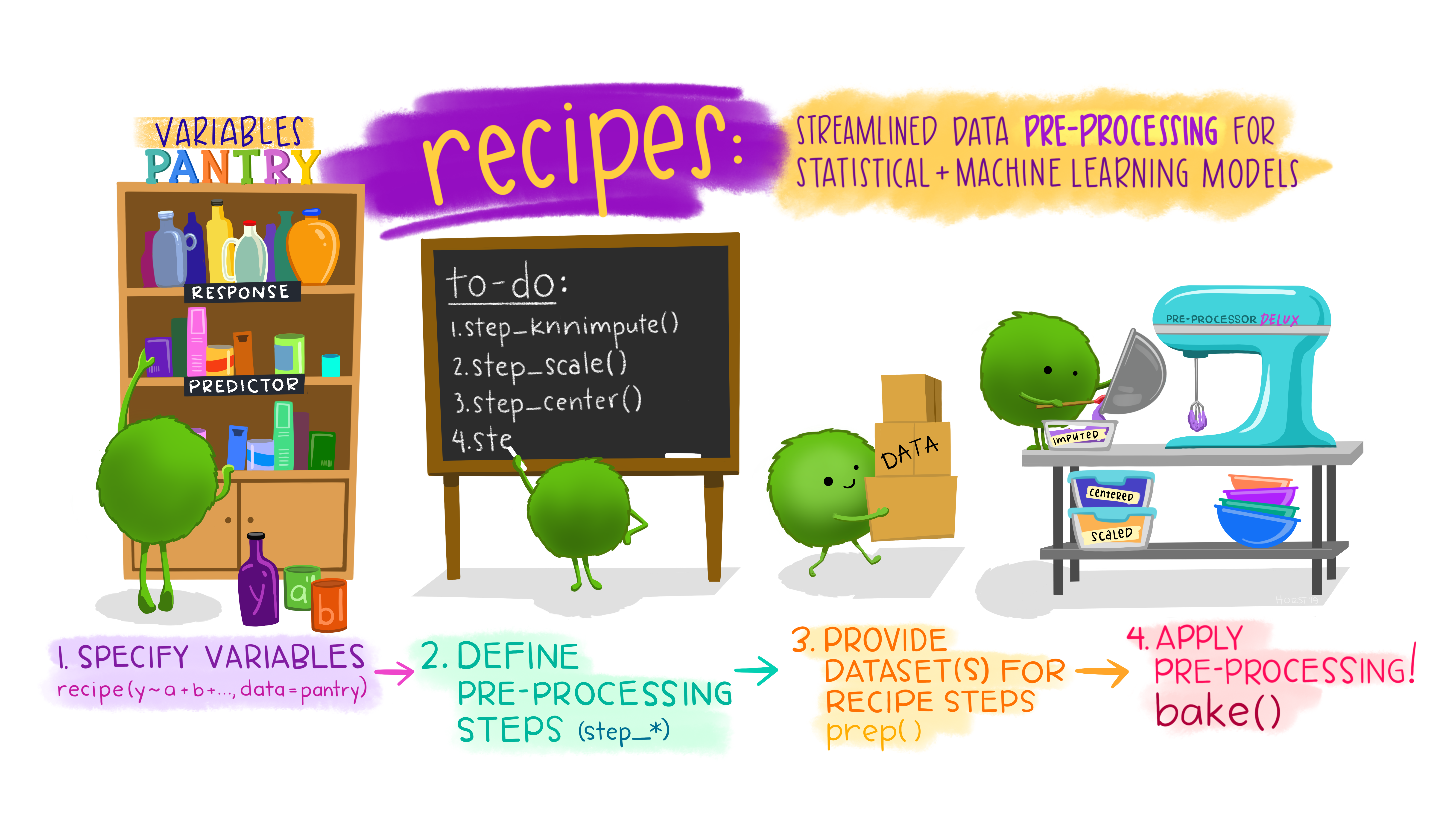
Understanding the Concept of a recipe in Data Preprocessing
In the tidymodels ecosystem, a recipe is a blueprint that outlines how to prepare your data for modeling. It’s a series of instructions or steps ( full list available here) that transform raw data into a format more suitable for analysis, ensuring that the preprocessing is systematic and reproducible. Here’s why recipes are pivotal in the data science workflow:
Standardization and Normalization: Recipes can include steps to standardize or normalize or transform numerical data, ensuring that variables are on comparable scales or have desired distributions (e.g., normal). Main functions:
step_log(): Applies log transformationstep_center(): Normalizes numeric columns by forcing mean = 0.step_scale(): Normalizes numeric columns by forcing sd = 1step_normalize(): Normalizes numeric columns by forcing mean = 0 & sd = 1.
Handling Missing Data: They allow you to specify methods for imputing missing values, ensuring the model uses a complete dataset for training. Main functions:
step_impute_median(): Imputes missing numeric values with the medianstep_impute_mean(): Imputes missing numeric values with the averagestep_impute_mode(): Imputes missing categorical values with the mode
Encoding Categorical Variables: Recipes describe how to convert categorical variables into a format that models can understand, typically through one-hot encoding or other encoding strategies. Main functions:
step_dummy(): Creates dummy variables for categorical predictorsstep_other(): Collapses infrequent factors into an “other” category
Feature Engineering: Recipe can include steps for creating new features from existing ones, enhancing the model’s ability to learn from the data. Main functions:
step_mutate(): Creates a new feature from an existing onestep_interact(): Creates interaction terms between features
Data Filtering and Columns Selection: They can also be used to select specific variables or filter rows based on certain criteria, tailoring the dataset to the modeling task. Main functions:
step_select(): Selects specific variables to retain in the datasetstep_slice(): Filters rows using their positionstep_filter(): Filters rows using logical conditions
Important
By defining these steps in a recipe, you create a reproducible set of transformations that can be applied to any dataset of the same structure and across multiple models.
This reproducibility is crucial for maintaining the integrity of your modeling process, especially when moving from a development environment to production.
Example: Creating a recipe for the ames dataset
Let’s create a recipe for the ames housing dataset, focusing on preprocessing steps that are commonly required for this type of data.
Note
Our goal is to predict house sale prices, so we’ll include steps to log-transform the target variable (to address skewness) and normalize the numerical predictors.

Define the recipe
Log-transform the Sale_Price to normalize its distribution
Normalize all numerical predictors
Prepare for modeling by converting factor/categorical variables into dummy variables
Do you notice the differences between ames and preprocessed_ames?
Warning
I showed you just a few columns affected by the recipe preprocessing steps. However, due to the
step_dummy(all_nominal_predictors())step, all the factor/categorical variables are converted from factor into dummies variables.Check the difference in the number of columns available in
amesandpreprocessed_amesto see the impact of that preprocessing step. You will see that such preprocessing step resulted in many more columns so always question if you need all the existing columns in your analysis or if you need to transform all of them into dummy variables.
Recap of the recipe steps
The ames_recipe outlines a series of preprocessing steps tailored to the ames dataset:
The
step_log()function applies a log transformation to theSale_Price, which is a common technique to normalize the distribution of the target variable in regression tasks.The
step_normalize()function centers and scales numerical predictors, ensuring they contribute equally to the model’s predictions.The
step_dummy()function converts categorical variables into a series of binary (0/1) columns, enabling models to incorporate this information.
By preparing the data with this recipe, we enhance the dataset’s suitability for predictive modeling, improving the potential accuracy and interpretability of the resulting models.
Important
It is critical that you verify that the preprocessing steps applied lead to the desired outcomes. For example, did the log transformation addressed the normality issue of your target variable?
Recipes in tidymodels provide a flexible and powerful way to specify and execute a series of data preprocessing steps, ensuring that your data science workflow is both efficient and reproducible.
Activity 1: Preprocessing with recipes. Write the code to complete the below tasks - 10 minutes
[Write code just below each instruction; finally use MS Teams R - Forum channel for help on the in class activities/homework or if you have other questions]
Standardize mean and sd of the Gr_Liv_Area, and impute missing values for Lot_Frontage with median, and for Garage_Type with mean.
What do you notice?
Important
If you prep and bake this recipe you will see an error. Garage type is not a numeric column so I can’t compute the average. I should use step_impute_mode.
Add to activity 1a the steps required to create dummy variables for the Neighborhood column, and to normalize the Year_Built column to force mean = 0.
Add to activity 1b the steps required to create an interaction term between the Overall_Qual and the Gr_Liv_Area columns and to standardize mean and sd of the Lot_Area variable.
Add to activity 1c the steps required to keep only the Sale_Price, Overall_Qual, Gr_Liv_Area and Year_Built columns. Moreover, slice the dataset to select only the first 500 rows.
Part 3: Building Models with parsnip in tidymodels
The parsnip package is a cornerstone of the tidymodels ecosystem designed to streamline and unify the process of model specification across various types of models and machine learning algorithms.
Unlike traditional approaches that require navigating the syntax and idiosyncrasies of different modeling functions and packages, parsnip abstracts this complexity into a consistent and intuitive interface. Here’s why parsnip stands out:
Unified Interface:
parsnip offers a single, cohesive syntax for specifying a wide range of models ( full list available here), from simple linear regression to complex ensemble methods and deep learning. This uniformity simplifies learning and reduces the cognitive load when switching between models or trying new methodologies. Main models:
Regression Models:
When to Use: Ideal for predicting continuous outcomes when the relationship between independent variables and the dependent variable is linear.
Example: Predicting house prices based on attributes like size (square footage), number of bedrooms, and age of the house.
When to Use: Useful when dealing with multicollinearity (independent variables are highly correlated) in your data or when you want to prevent overfitting by adding a penalty (L2 regularization) to the size of coefficients.
Example: Predicting employee salaries using a range of correlated features like years of experience, level of education, and job role.
When to Use: Similar to Ridge regression but can shrink some coefficients to zero, effectively performing variable selection (L1 regularization). Useful for models with a large number of predictors, where you want to identify a simpler model with fewer predictors.
Example: Selecting the most impactful factors affecting the energy efficiency of buildings from a large set of potential features.
Classification & Tree-Based Models
Important
Tree-based models can be used also for regression. We will see later how to change their purpose based on the analysis objective.
When to Use: Suited for binary classification problems where you predict the probability of an outcome that can be one of two possible states.
Example: Determining whether an email is spam or not based on features like the frequency of certain words, sender reputation, and email structure.
When to Use: Good for classification and regression with a dataset that includes non-linear relationships. Decision trees are interpretable and can handle both numerical and categorical data.
Example: Predicting customer churn based on a variety of customer attributes such as usage patterns, service complaints, and demographic information.
When to Use: When you require a robust predictive model for both regression and classification that can automatically handle missing values and does not require scaling of data. It builds trees in a sequential manner, minimizing errors from previous trees.
Example: Predicting with high accuracy complex outcomes such as future sales amounts across different stores and products.
When to Use: Suitable for scenarios where high accuracy is crucial, and the model can handle being a “black box.” Works well for both classification and regression tasks and is robust against overfitting.
Example: Diagnosing diseases from patient records where there’s a need to consider a vast number of symptoms and test results.
Deep Learning: Neural Network
When to Use: Best for capturing complex, nonlinear relationships in high-dimensional data. Neural networks excel in tasks like image recognition, natural language processing, and time series prediction.
Example: Recognizing handwritten digits where the model needs to learn from thousands of examples of handwritten digits.
What we learned from the above?
Each of these model functions can be specified with parsnip’s unified interface, allowing you to easily switch between them or try new models with minimal syntax changes. The choice of model and the specific parameters/arguments (penalty, mtry, trees, etc.) should be guided by the nature of your data, the problem at hand, and possibly iterative model tuning processes like training-test sampling and cross-validation.
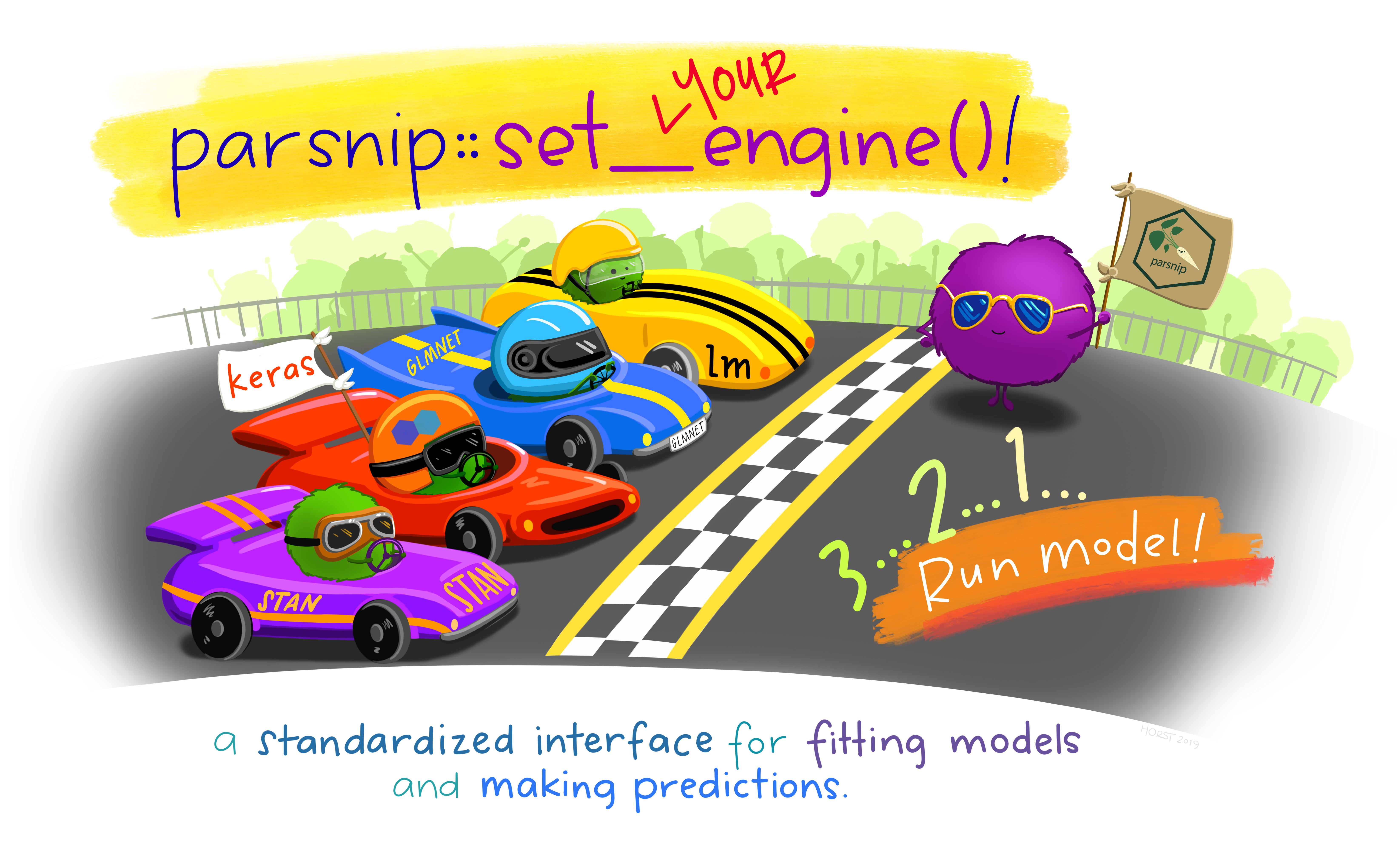
Engine Independence: Behind the scenes, many models can be fitted using different computational engines (e.g., lm, glmnet, ranger). parsnip allows you to specify the model once and then choose the computational engine separately, providing flexibility and making it easy to compare the performance of different implementations.
Integration with tidymodels: parsnip models seamlessly integrate with other tidymodels packages, such as
recipesfor data preprocessing,workflowsfor bundling preprocessing and modeling steps, andtunefor hyperparameter optimization.
Starting Simple: Specifying a Linear Regression Model Using parsnip
Linear regression is one of the most fundamental statistical and machine learning methods, used for predicting a continuous outcome based on one or more predictors. Let’s specify a linear regression model using parsnip for the ames housing dataset, aiming to predict the sale price of houses from their characteristics.
In this specification:
linear_reg()initiates the specification of a linear regression model. At this stage, we’re defining the type of model but not yet fitting it to data.set_engine("lm")selects the computational engine to use for fitting the model. Here, we use “lm”, which stands for linear models, a base R function well-suited for fitting these types of models.set_mode("regression")indicates that we are performing a regression task, predicting a continuous outcome.
Important
- This process outlines the model we intend to use without binding it to specific data. The next steps typically involve integrating the prepared data (using a recipe), fitting the model to training data, and evaluating its performance.
parsnip’s design makes these steps straightforward and consistent across different types of models, enhancing the reproducibility and scalability of your modeling work.
Through the abstraction provided by parsnip, model specification becomes not only more straightforward but also more adaptable to different contexts and needs, facilitating a smoother workflow in predictive modeling projects.
Activity 2: Exploring modeling with parsnip. - 10 minutes:
[Write code just below each instruction; finally use MS Teams R - Forum channel for help on the in class activities/homework or if you have other questions]
Define a linear regression model (lm) predicting Sale_Price using Lot_Area
What do you notice?
Specify a linear regression model (lm) predicting Sale_Price using Gr_Liv_Area and Lot_Area
What do you notice? How different it is from the model in Activity 2a?
Define a decision tree model to predict Sale_Price using Lot_Area and Year_Built.
What do you notice?
Specify a decision tree model to predict Sale_Price using Gr_Liv_Area and Lot_Area.
What do you notice? How does it differ to the model in Activity 2c?
Caution
As you probably noticed the specification of the models in 2a and 2b and the one of the models in 2c and 2d is identical.
Important
Why and how is that possible? The secret is that parsnip doesn’t require specifications of variables or formulas to be used in/by the models. That piece of information is acquired when we use workflows and we actually fit the models. Because of this, it is extremely easy to reuse defined models across different datasets and analyses.
Part 4: Integrating Preprocessing and Modeling with workflows
The workflows package is a powerful component of the tidymodels ecosystem designed to streamline the modeling process. It provides a cohesive framework that binds together preprocessing steps (recipes) and model specifications (parsnip) into a single, unified object. This integration enhances the modeling workflow by ensuring consistency, reproducibility, and efficiency.
Key Advantages of Using workflows:
Unified Process: By encapsulating both preprocessing (e.g., feature engineering, normalization) and modeling within a single object,
workflowssimplifies the execution of the entire modeling pipeline. This unified approach reduces the risk of mismatches or errors between the data preprocessing and modeling stages.Reproducibility:
workflowsmakes your analysis more reproducible by explicitly linking preprocessing steps to the model. This linkage ensures that anyone reviewing your work can see the complete path from raw data to model outputs.Flexibility and Efficiency: It allows for easy experimentation with different combinations of preprocessing steps and models. Since preprocessing and model specification are encapsulated together, switching out components to test different hypotheses or improve performance becomes more streamlined.
Building and Fitting a Model Using workflows
To demonstrate the practical application of workflows, let’s consider the ames housing dataset, where our goal is to predict house sale prices based on various features. We’ll use the linear regression model specified with parsnip and the preprocessing recipe developed with recipes.
Warning
Make sure that ames_recipe, a preprocessing steps object created with recipes, is in your environment (check it to be true by running ls()) and that also linear_mod, a linear regression model specified with parsnip, is available in your environment
Create the workflow by combining the recipe and model
Fit the workflow to the Ames housing data
In this process:
We start by creating a new
workflowobject, to which we add our previously defined preprocessing recipe (ames_recipe) and linear regression model (linear_mod).The
add_recipe()andadd_model()functions are used to incorporate the preprocessing steps and model specification into the workflow, respectively.The
fit()function is then used to apply this workflow to theamesdataset, executing the preprocessing steps on the data before fitting the specified model.The result is a fitted model object that includes both the preprocessing transformations and the model’s learned parameters, ready for evaluation or prediction on new data.
This example underscores how workflows elegantly combines data preprocessing and model fitting into a cohesive process, streamlining the journey from raw data to actionable insights.
By leveraging workflows, data scientists can maintain a clear, organized, and efficient modeling pipeline. workflows epitomizes the philosophy of tidymodels in promoting clean, understandable, and reproducible modeling practices.
Through its structured approach to integrating preprocessing and modeling, workflows facilitates a seamless transition across different stages of the predictive modeling process.
Note
We will ignore the results interpretation for now because we don’t know how to evaluate the models yet but you can see how simple it is to create and run a modeling workflow.
Activity 3: Streamline Modeling with Workflow. - 15 minutes
[Write code just below each instruction; finally use MS Teams R - Forum channel for help on the in class activities/homework or if you have other questions]
Define a recipe (“recipe_3a”) for the following preprocessing steps: standardize Gr_Liv_Area and encode Neighborhood as dummy variables. Specify a linear regression model using the ‘lm’ engine (lm_reg_3a). Create a workflow, add the recipe_3a recipe and the lm_reg_3a model, then fit the workflow to the ames data.
Define a recipe (“recipe_3b”) for the following preprocessing steps: compute a new “Total_flr_SF” variable equal to First_Flr_SF + Second_Flr_SF and encode MS_SubClass to make sure that infrequent values fall inside the other category. Specify a classification decision tree model (“tree_3b”). Create a workflow, add the recipe_3b recipe and the tree_3b model, then fit the workflow to the ames data.
Important
While the instructions asked you to use classification as mode, the dependent variable is numerical so we can’t use it. We should use regression. Finally tidy() can’t be used to visualize the decision tree results.
Define a recipe (“recipe_3c”) for the following preprocessing steps: scale ‘Lot_Area’ and sample only 500 rows. Specify a linear regression model using ‘glmnet’ engine (“glmnet_reg_3c”) using penalty = 0.1 and mixture = 0. Create a workflow, add the recipe_3c recipe and the glmnet_reg_3c model, then fit the workflow to the ames data.
Important
If you use regularized regressions (lasso or ridge) you need more than 1 variable so I added Gr_Liv_Area in the recipe_3c_revised to get rid of the error. The objective of the activities is to expose you to this type of errors/issues. So, if you use recipe_3c_revised in the above workflow you will get results and not this error message: “Error in glmnet::glmnet(x = maybe_matrix(x), y = y, alpha = ~1, family =”gaussian”) : x should be a matrix with 2 or more columns”
Define a recipe (“recipe_3d”) for the following preprocessing steps: log transform Lot_Frontage and encode all nominal variables as dummy variables. Specify a decision tree model (“tree_mod_3d”). Create a workflow, add the recipe_3d recipe and the tree_mod_3d model, then fit the workflow to the ames data.
Important
This is enough for our first coding modeling class with tidymodels. More to come in the next weeks but please make sure you understand everything we have covered so far! Please reach out for help and ask clarifications if needed. We are here to help ;-)